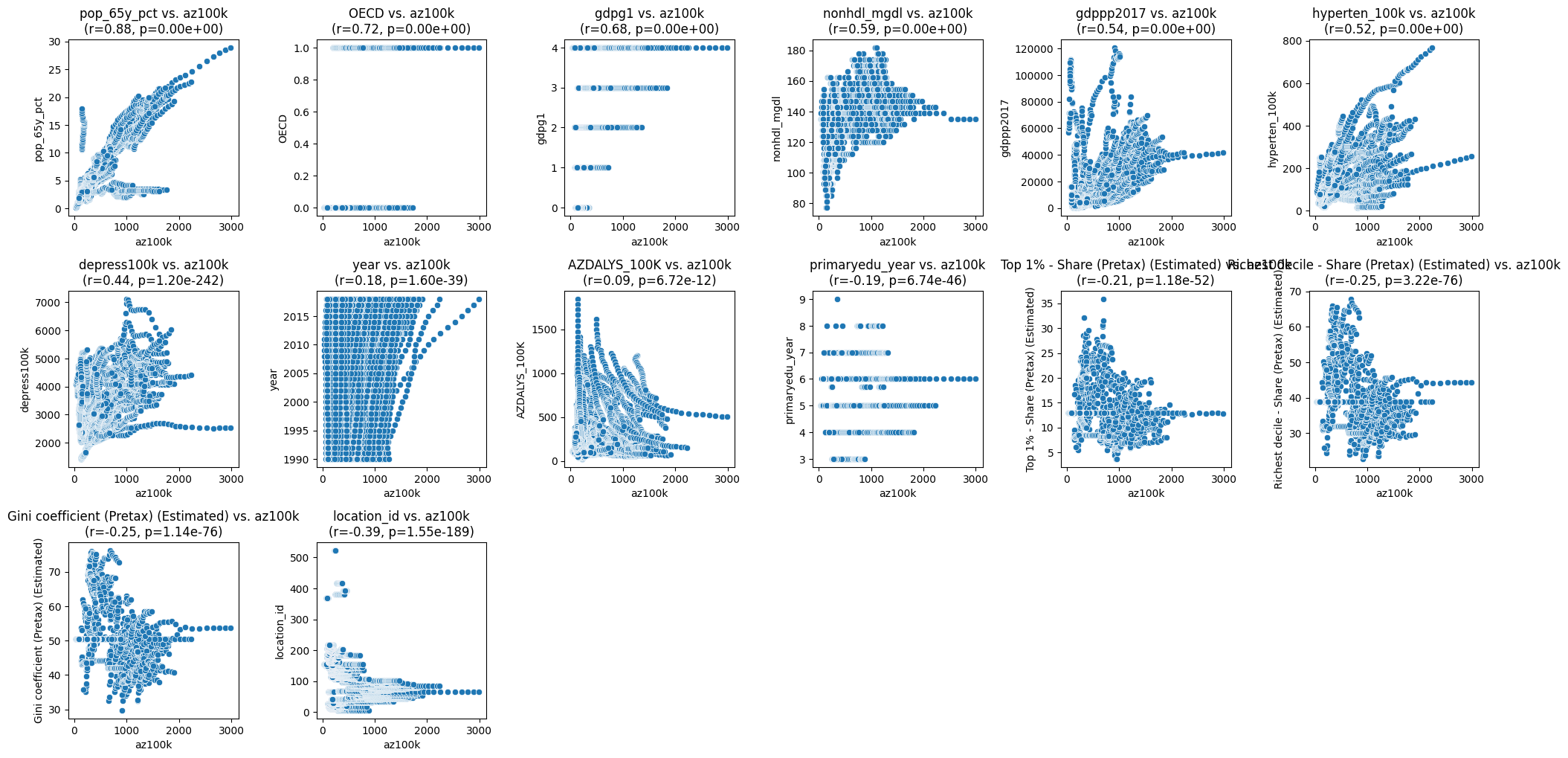
Pearson Correlation with AZ PVR and corresponding P-values:
                                             Pearson Correlation  \
pop_65y_pct                                             0.878693
OECD                                                    0.715244
gdpg1                                                   0.675784
nonhdl_mgdl                                             0.589307
gdppp2017                                               0.540096
hyperten_100k                                           0.519576
depress100k                                             0.435002
year                                                    0.179636
AZDALYS_100K                                            0.094284
primaryedu_year                                        -0.193938
Top 1% - Share (Pretax) (Estimated)                    -0.207960
Richest decile - Share (Pretax) (Estimated)            -0.250316
Gini coefficient (Pretax) (Estimated)                  -0.251049
location_id                                            -0.388319

                                                   P-value
pop_65y_pct                                   0.000000e+00
OECD                                          0.000000e+00
gdpg1                                         0.000000e+00
nonhdl_mgdl                                   0.000000e+00
gdppp2017                                     0.000000e+00
hyperten_100k                                 0.000000e+00
depress100k                                  1.196912e-242
year                                          1.602392e-39
AZDALYS_100K                                  6.723790e-12
primaryedu_year                               6.743125e-46
Top 1% - Share (Pretax) (Estimated)           1.176397e-52
Richest decile - Share (Pretax) (Estimated)   3.223273e-76
Gini coefficient (Pretax) (Estimated)         1.141362e-76
location_id                                  1.552886e-189
import pandas as pd
import numpy as np
import matplotlib.pyplot as plt
import seaborn as sns
from scipy.stats import pearsonr
# Select only numerical columns
numerical_data = data.select_dtypes(include=[np.number])

# Handle NaN and infinite values by replacing them with the mean of the column
numerical_data = numerical_data.apply(lambda x: np.where(np.isfinite(x), x, np.nan))
numerical_data = numerical_data.apply(lambda x: x.fillna(x.mean()), axis=0)

# Calculate Pearson correlation with target variable 'az100k'
target_variable = 'az100k'
correlation_results = {}

for column in numerical_data.columns:
    if column != target_variable:
        correlation, p_value = pearsonr(numerical_data[target_variable], numerical_data[column])
        correlation_results[column] = {'Pearson Correlation': correlation, 'P-value': p_value}

# Convert results to DataFrame for better visualization
correlation_df = pd.DataFrame.from_dict(correlation_results, orient='index')
correlation_df = correlation_df.sort_values(by='Pearson Correlation', ascending=False)

print("Pearson Correlation with Close_TAIEX and corresponding P-values:")
print(correlation_df)

# Plot scatter plots for each explanatory variable vs. az100k
plt.figure(figsize=(20, 20))
for i, column in enumerate(correlation_df.index):
    plt.subplot(6, 6, i + 1)  # Adjust the number of rows and columns based on the number of variables
    sns.scatterplot(x=numerical_data[target_variable], y=numerical_data[column])
    plt.title(f'{column} vs. {target_variable}\n(r={correlation_df.loc[column, "Pearson Correlation"]:.2f}, p={correlation_df.loc[column, "P-value"]:.2e})')
    plt.xlabel(target_variable)
    plt.ylabel(column)
plt.tight_layout()
plt.show()