
Close_TAIEX -N.Scatter Plot Matrix_0630


import pandas as pd
import numpy as np
import matplotlib.pyplot as plt
import seaborn as sns
from scipy.stats import pearsonr

# Mount Google Drive
from google.colab import drive
drive.mount('/content/drive', force_remount=True)

# Load the data
file_path = '/content/drive/My Drive/MSCI_Taiwan_30_data.csv'
data = pd.read_csv(file_path)

# Select only numerical columns
numerical_data = data.select_dtypes(include=[np.number])

# Handle NaN and infinite values by replacing them with the mean of the column
numerical_data = numerical_data.apply(lambda x: np.where(np.isfinite(x), x, np.nan))
numerical_data = numerical_data.apply(lambda x: x.fillna(x.mean()), axis=0)

# Calculate Pearson correlation with target variable 'Close_TAIEX'
target_variable = 'Close_TAIEX'
correlation_results = {}

for column in numerical_data.columns:
    if column != target_variable:
        correlation, p_value = pearsonr(numerical_data[target_variable], numerical_data[column])
        correlation_results[column] = {'Pearson Correlation': correlation, 'P-value': p_value}

# Convert results to DataFrame for better visualization
correlation_df = pd.DataFrame.from_dict(correlation_results, orient='index')
correlation_df = correlation_df.sort_values(by='Pearson Correlation', ascending=False)

print("Pearson Correlation with Close_TAIEX and corresponding P-values:")
print(correlation_df)

# Plot scatter plots for each explanatory variable vs. Close_TAIEX
plt.figure(figsize=(20, 20))
for i, column in enumerate(correlation_df.index):
    plt.subplot(6, 6, i + 1)  # Adjust the number of rows and columns based on the number of variables
    sns.scatterplot(x=numerical_data[target_variable], y=numerical_data[column])
    plt.title(f'{column} vs. {target_variable}\n(r={correlation_df.loc[column, "Pearson Correlation"]:.2f}, p={correlation_df.loc[column, "P-value"]:.2e})')
    plt.xlabel(target_variable)
    plt.ylabel(column)
plt.tight_layout()
plt.show()
import pandas as pd import yfinance as yf import ta from datetime import datetime
Mounted at /content/drive
Pearson Correlation with Close_TAIEX and corresponding P-values:
Pearson Correlation P-value
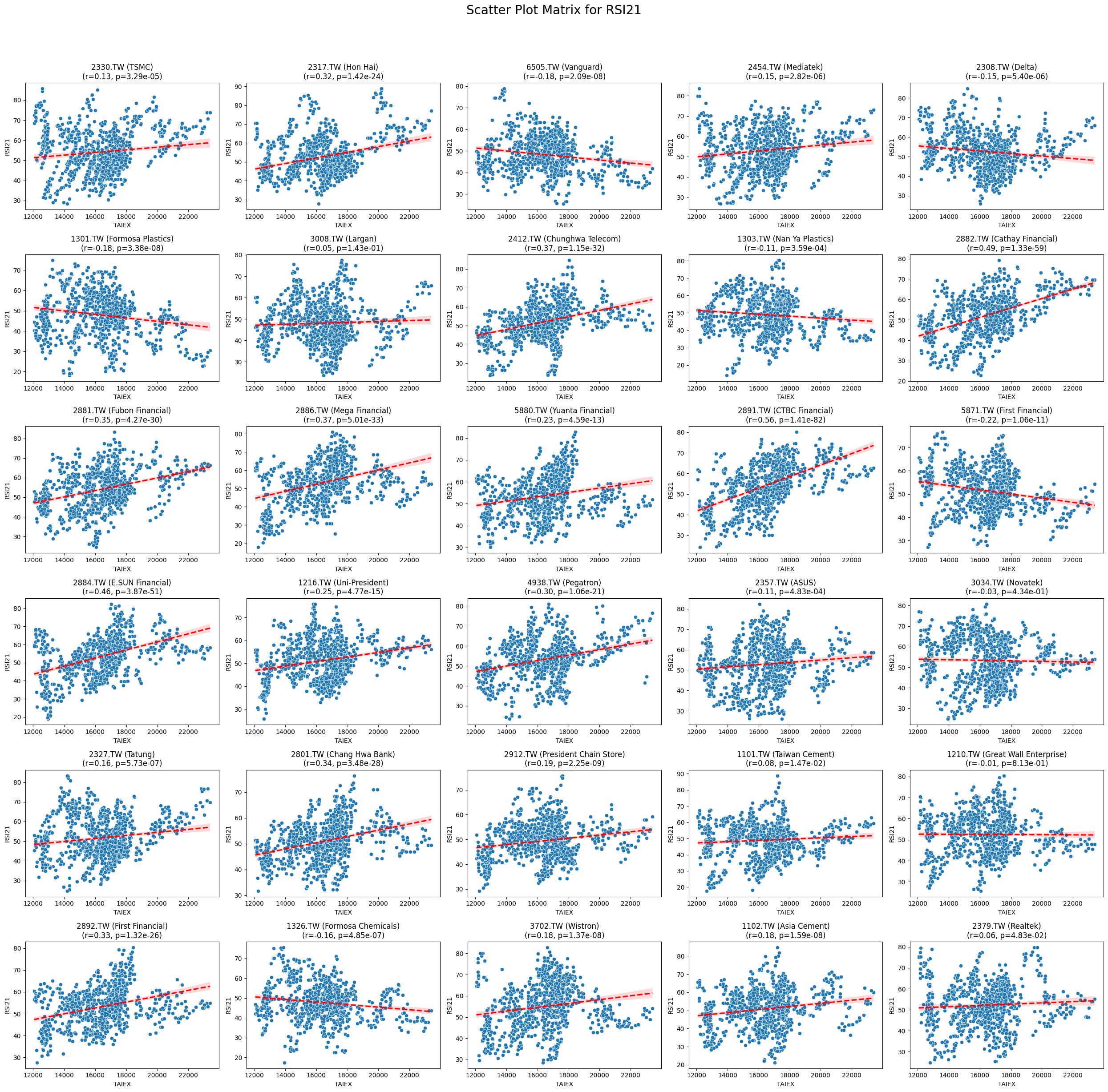
RSI21 0.181235 1.788855e-239
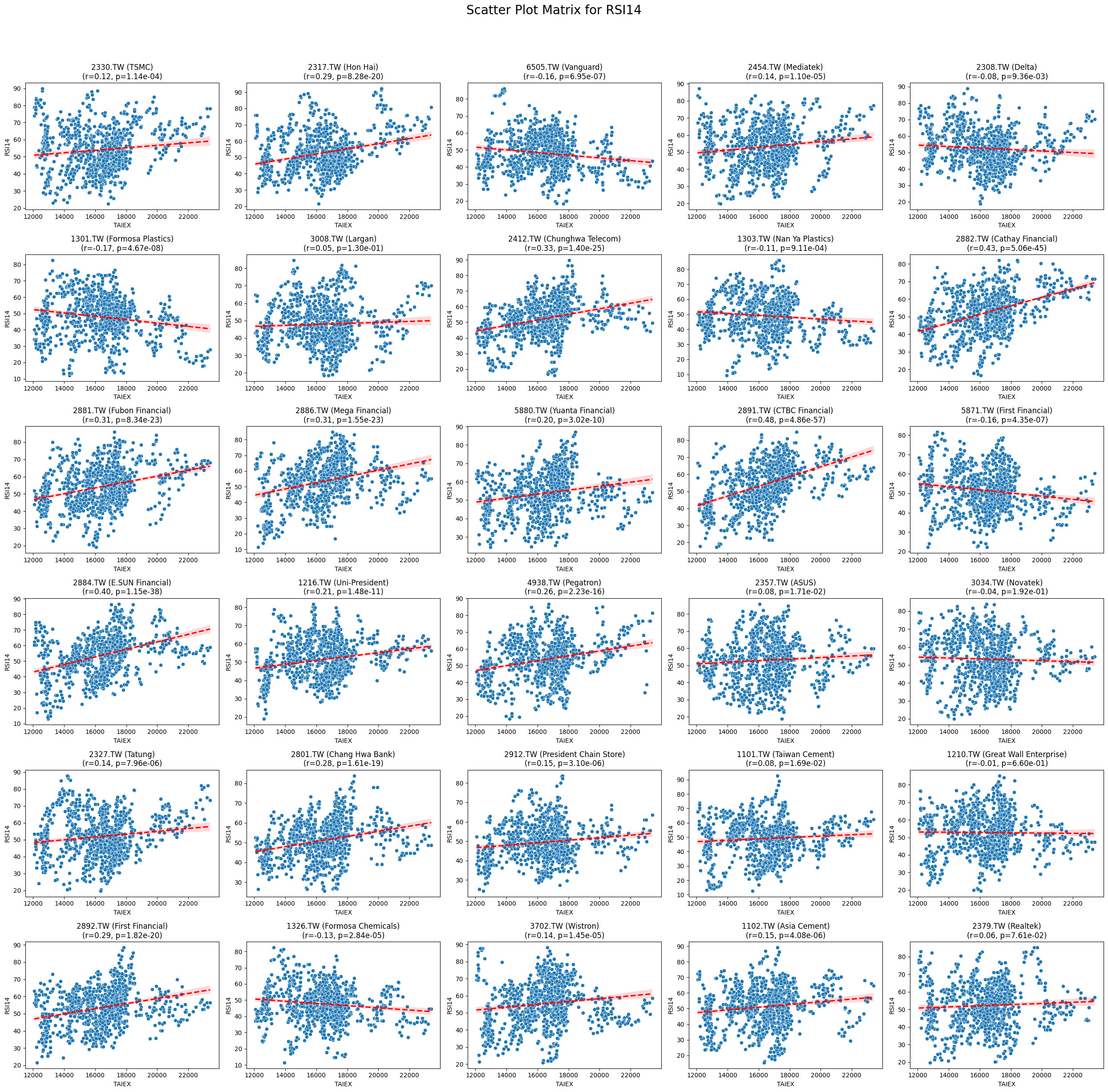
RSI14 0.149536 7.892582e-163
CMO14 0.097049 2.915690e-69
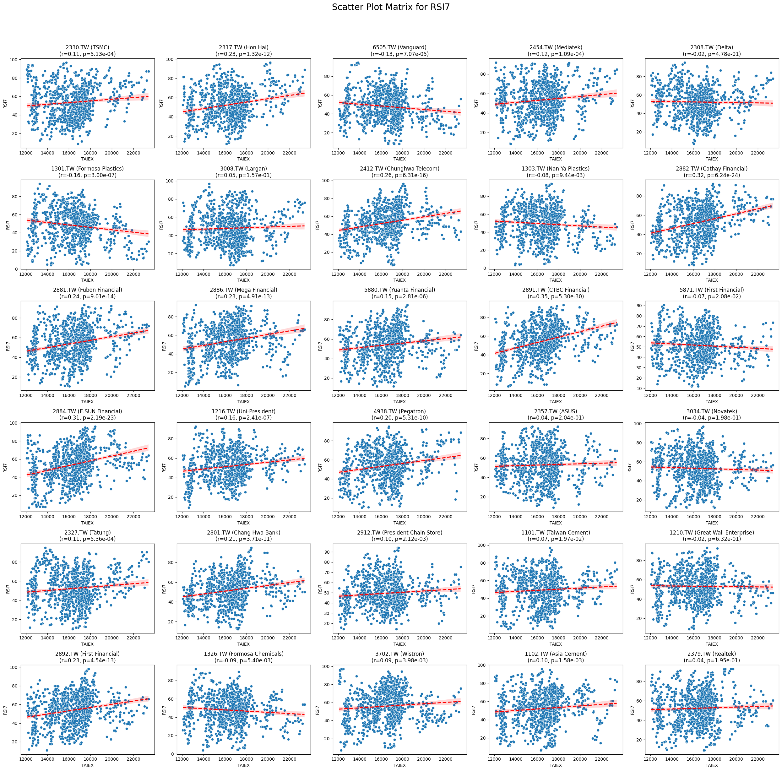
RSI7 0.094208 2.352703e-65
Aroon Up 0.092640 3.003308e-63
CCI20 0.085391 5.606595e-54
MACD Line 0.080482 3.944215e-48
Signal Line 0.079971 1.530058e-47
%D 0.065723 1.223437e-32
%K 0.062314 1.670302e-29
WILLR14 0.062314 1.670302e-29
Market Return 0.053534 3.417693e-22
Adj_Close 0.040832 1.508200e-13
Lower Band 0.025166 5.331465e-06
Stock Return 0.024956 6.379107e-06
Low 0.022923 3.390795e-05
Close_MSCI 0.022754 3.870897e-05
Open 0.022309 5.473519e-05
MA7 0.022306 5.485074e-05
High 0.022106 6.395461e-05
Middle Band 0.021395 1.092130e-04
MA21 0.021350 1.128899e-04
MA50 0.020800 1.688435e-04
MA100 0.018208 9.919776e-04
Upper Band 0.018121 1.049533e-03
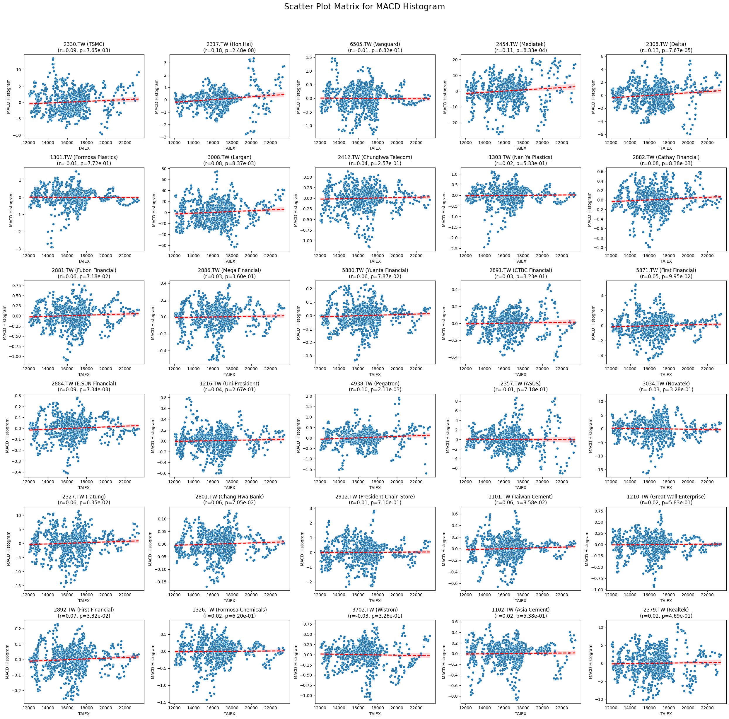
MACD Histogram 0.012237 2.691003e-02
Volume -0.014191 1.028059e-02
Band Width -0.021713 8.609264e-05
Aroon Down -0.081898 8.808426e-50
Beta_120 -0.124150 1.815258e-112
Beta_60 -0.164698 1.474482e-197import pandas as pd import yfinance as yf import ta from datetime import datetime
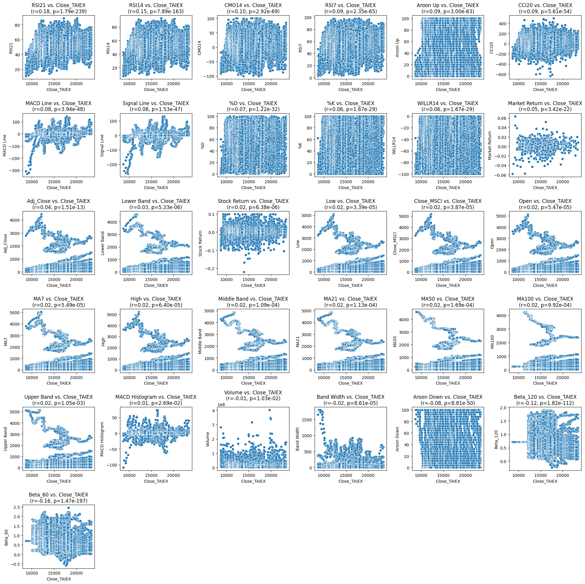
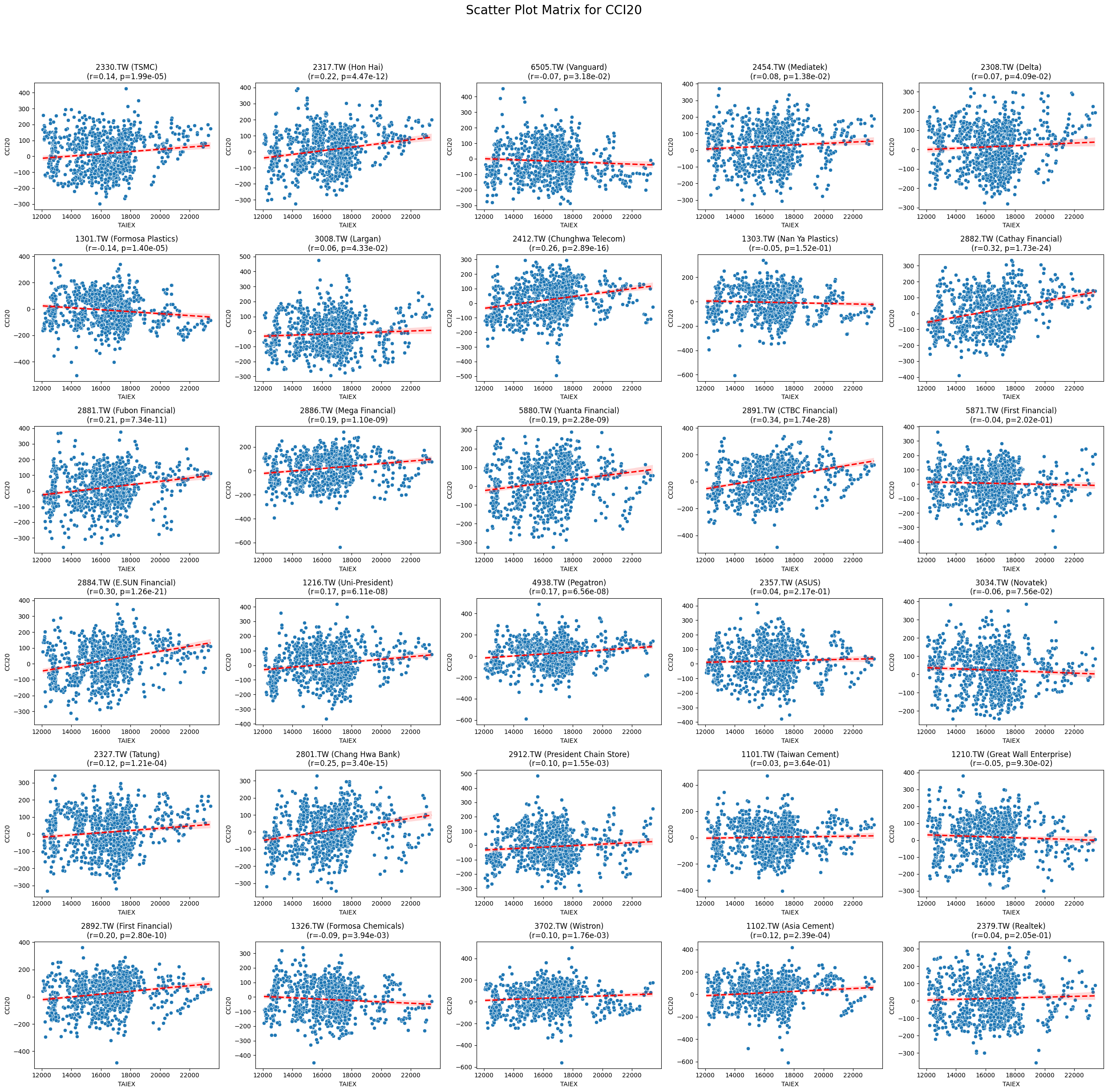
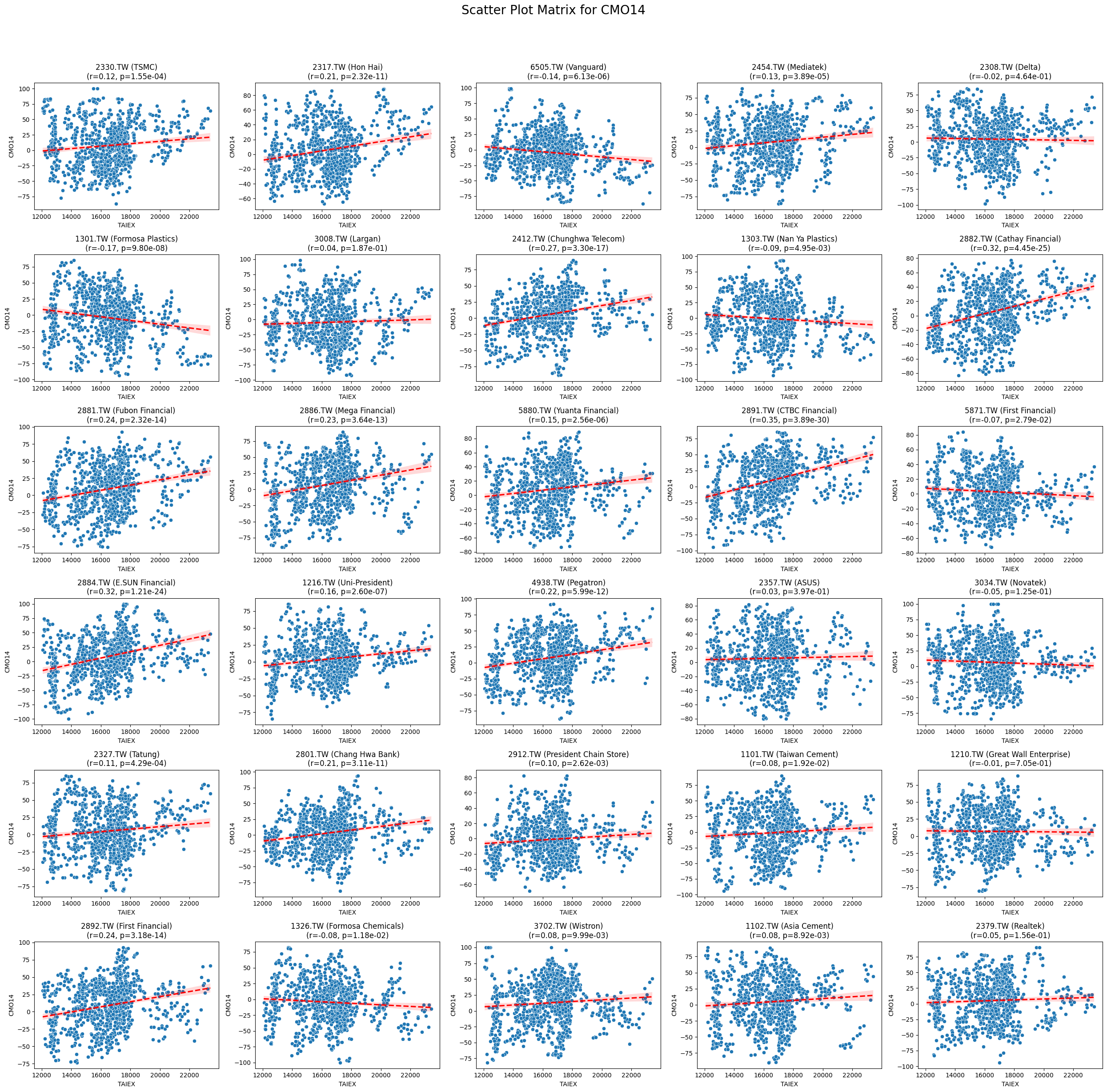
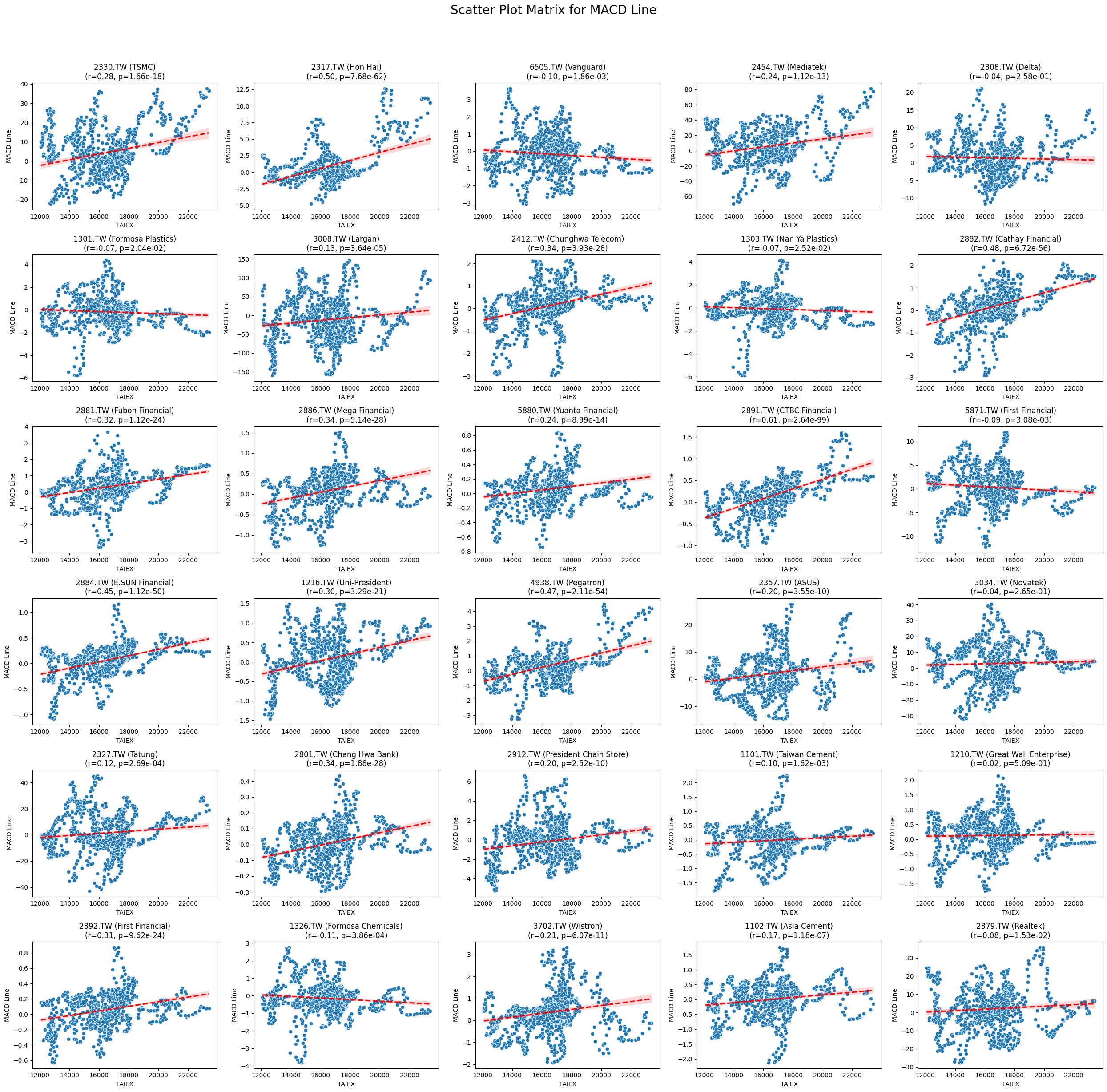
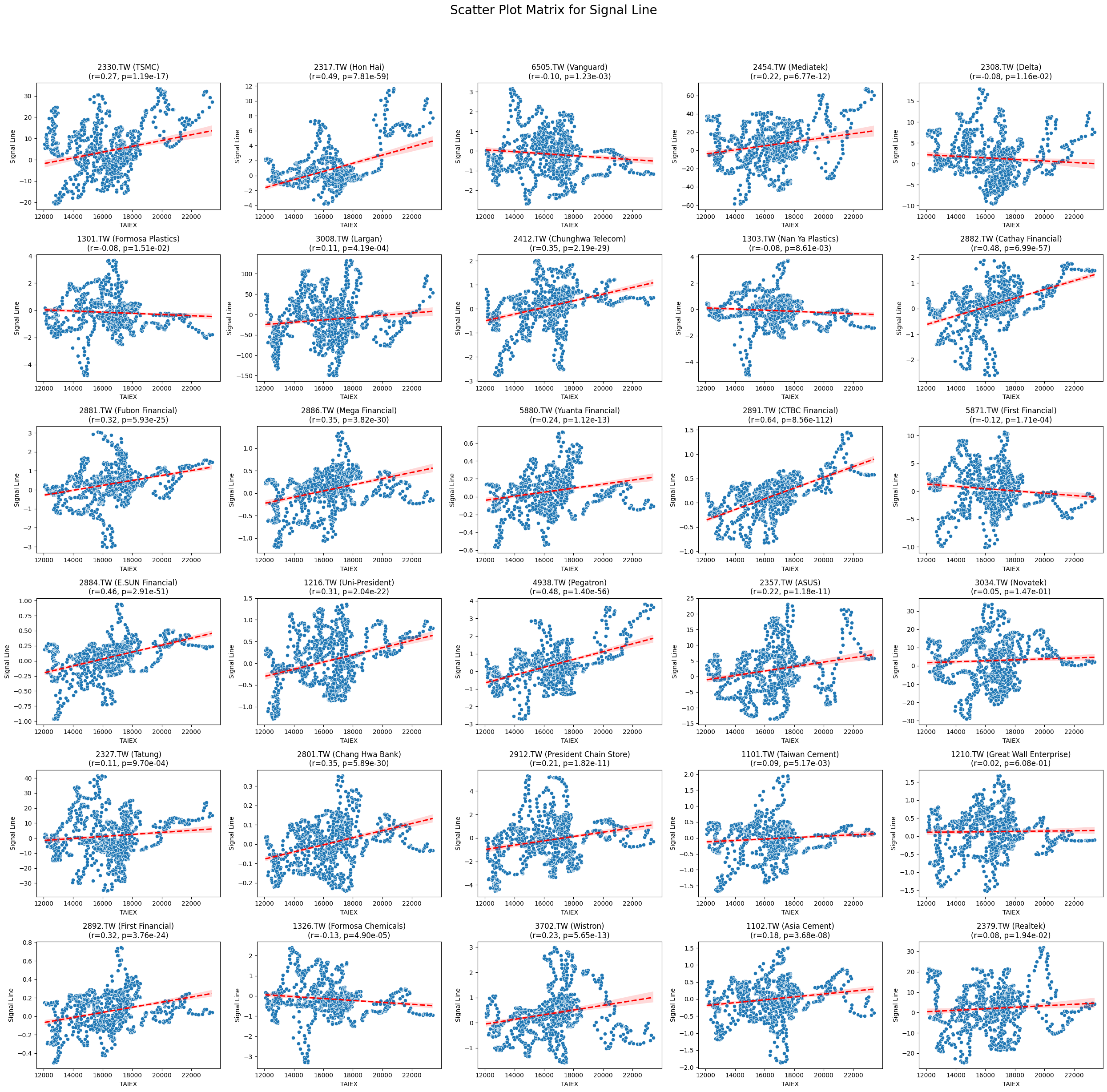
將相關技術指標分為微弱相關、正相關和負相關的表格,包括它們的相關係數(r)和 p 值:
類別指標r 值p 值微弱相關RSI21-0.017.19e-239RSI140.037.19e-168RSI7-0.092.73e-56Aroon Up0.039.03e-63Market Return0.092.43e-22Adj Close0.041.15e-13Lower Band0.035.33e-06Stock Return0.023.16e-06Low0.023.39e-05Close MSCI0.023.78e-05Open0.025.47e-05MA70.024.95e-05High0.026.46e-05Middle Band0.029.96e-04MA210.021.34e-04MA500.021.96e-04MA100.029.92e-04Upper Band0.025.05e-03MACD Histogram0.013.10e-02Band Width-0.028.16e-05正相關RSI140.037.19e-168CCI200.099.15e-54MACD Line0.051.11e-45Signal Line0.051.71e-42WILLR140.091.67e-29負相關CMO14-0.192.92e-69RSI7-0.092.73e-56%D-0.071.12e-29%K-0.061.47e-29Aroon Down-0.088.18e-50Beta 120-0.121.82e-112
變數分群的討論
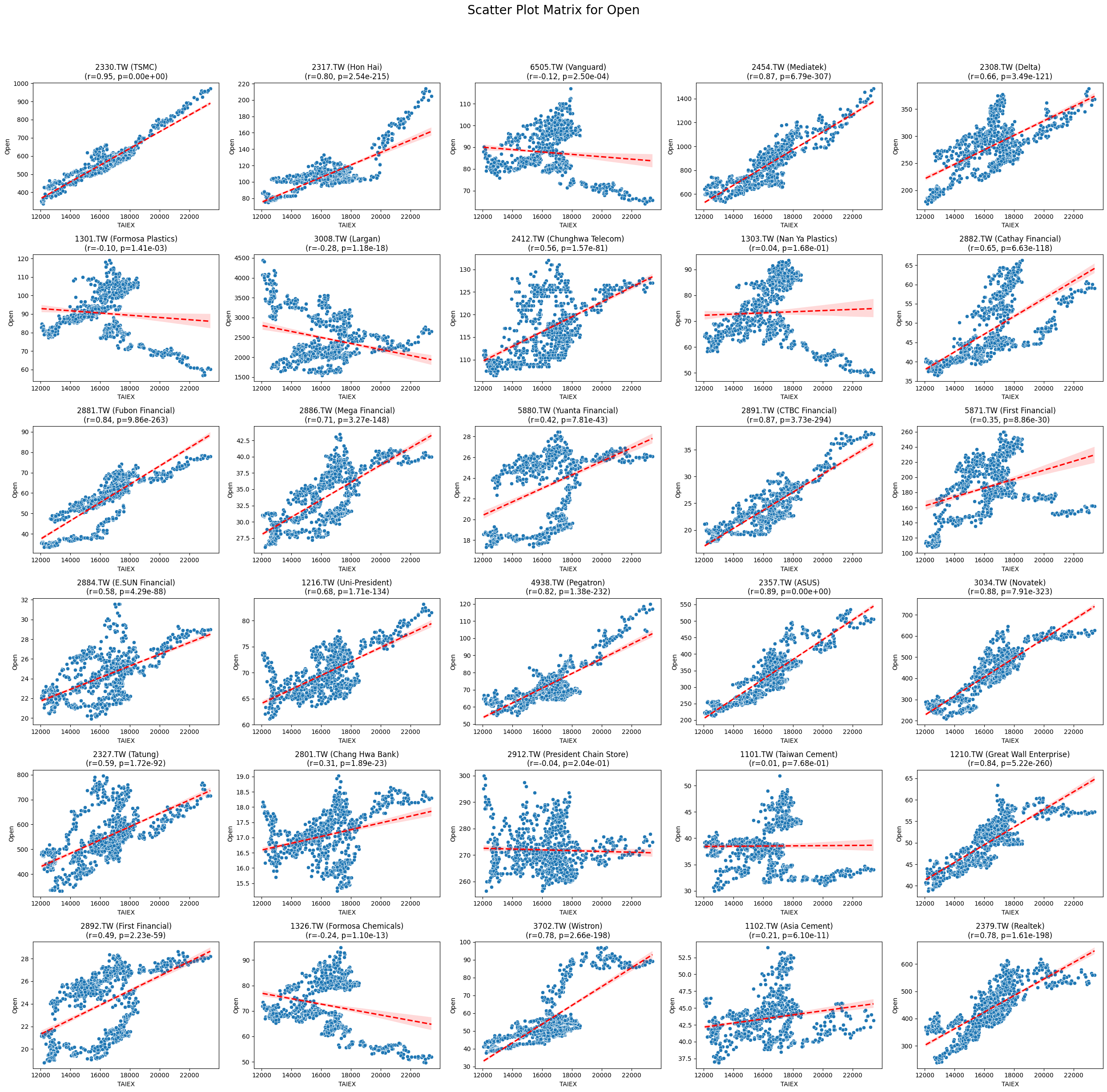
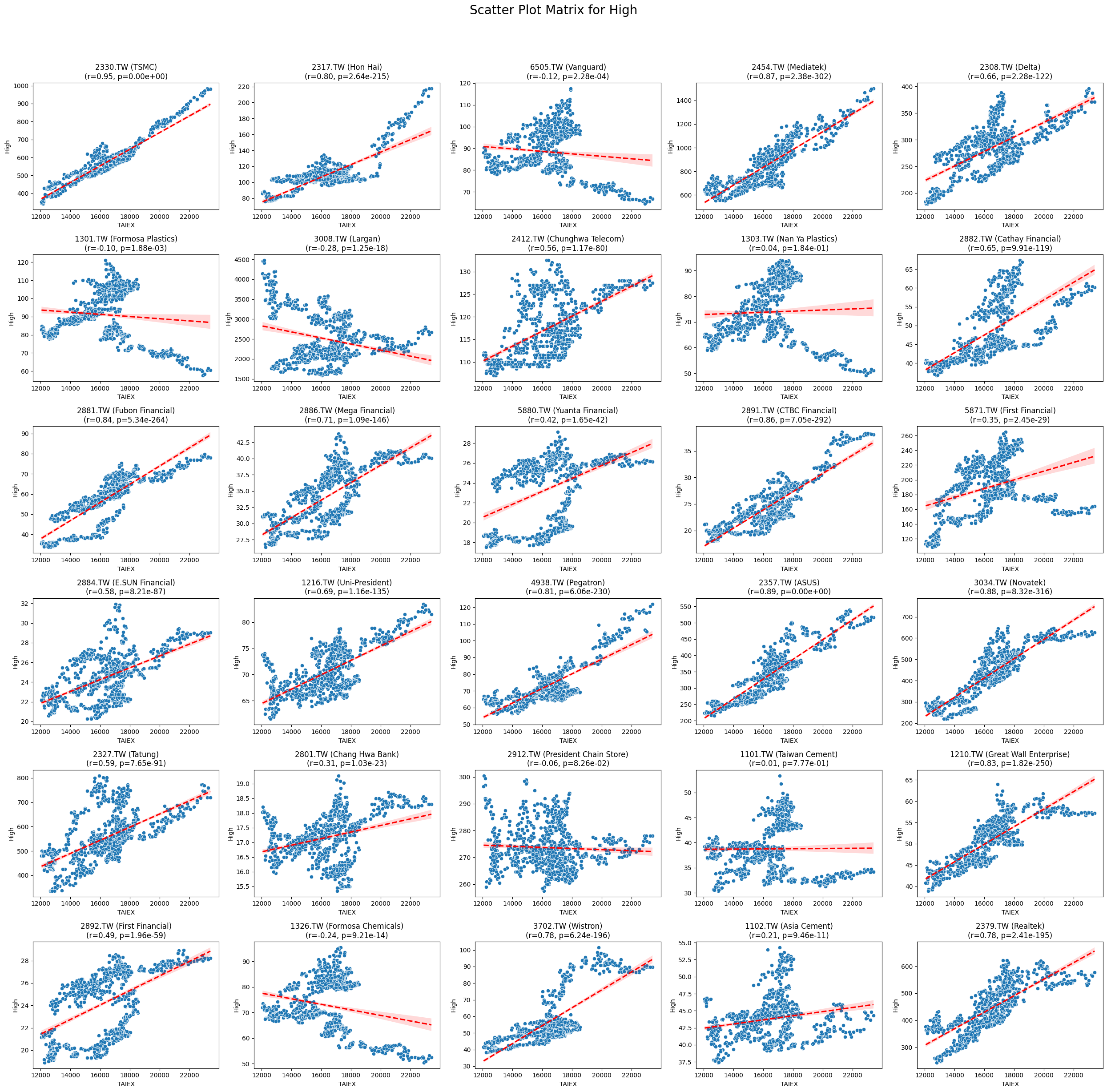
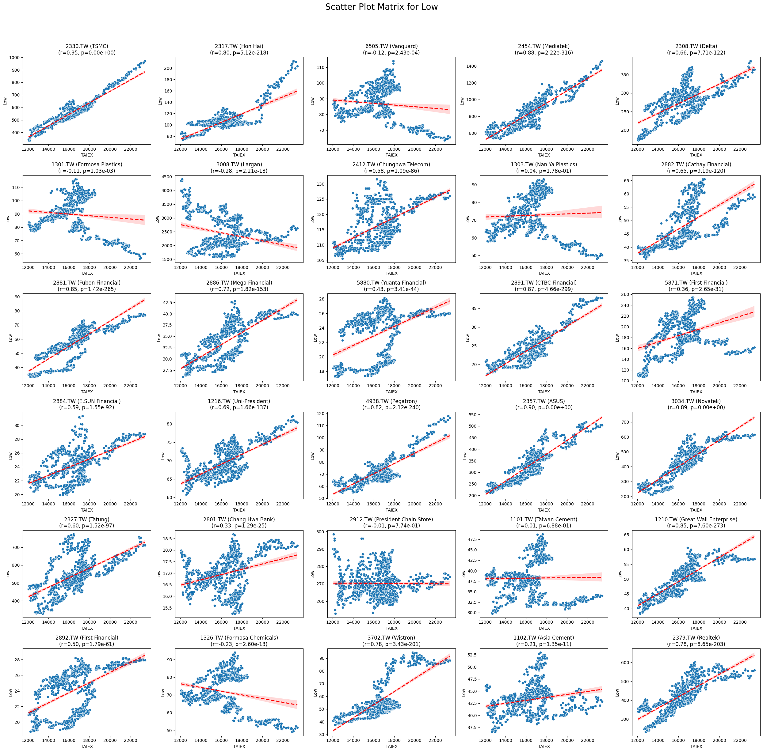
OPEN_High_Low_Close


Code
import pandas as pd
import numpy as np
import matplotlib.pyplot as plt
import seaborn as sns
from scipy.stats import pearsonr
# Mount Google Drive
from google.colab import drive
drive.mount('/content/drive', force_remount=True)
# Load the data
file_path = '/content/drive/My Drive/MSCI_Taiwan_30_data.csv'
data = pd.read_csv(file_path)
# Convert 'Date' column to datetime
data['Date'] = pd.to_datetime(data['Date'], format='%Y/%m/%d')
# Define the target variable
target_variable = 'Close_TAIEX'
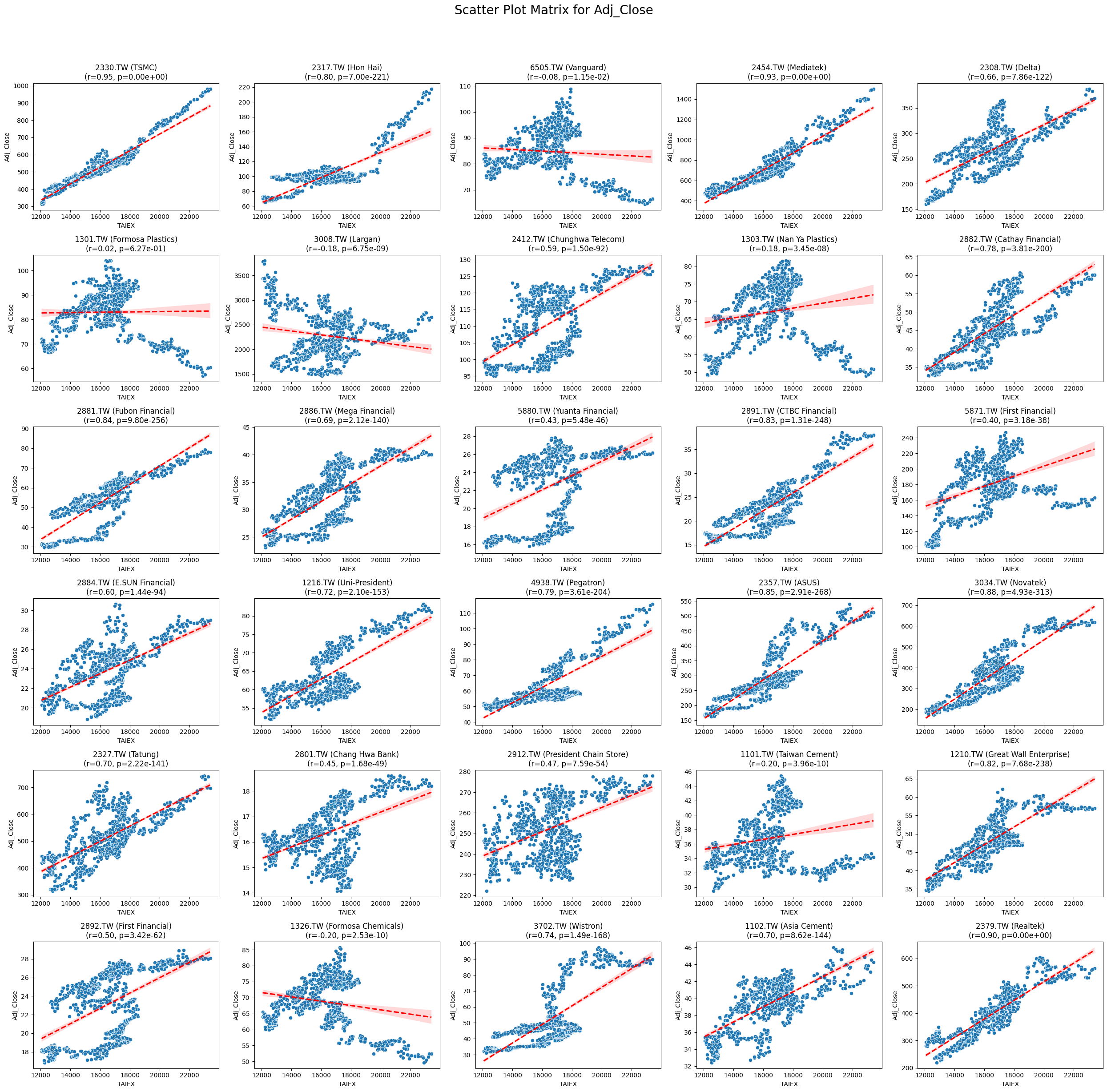
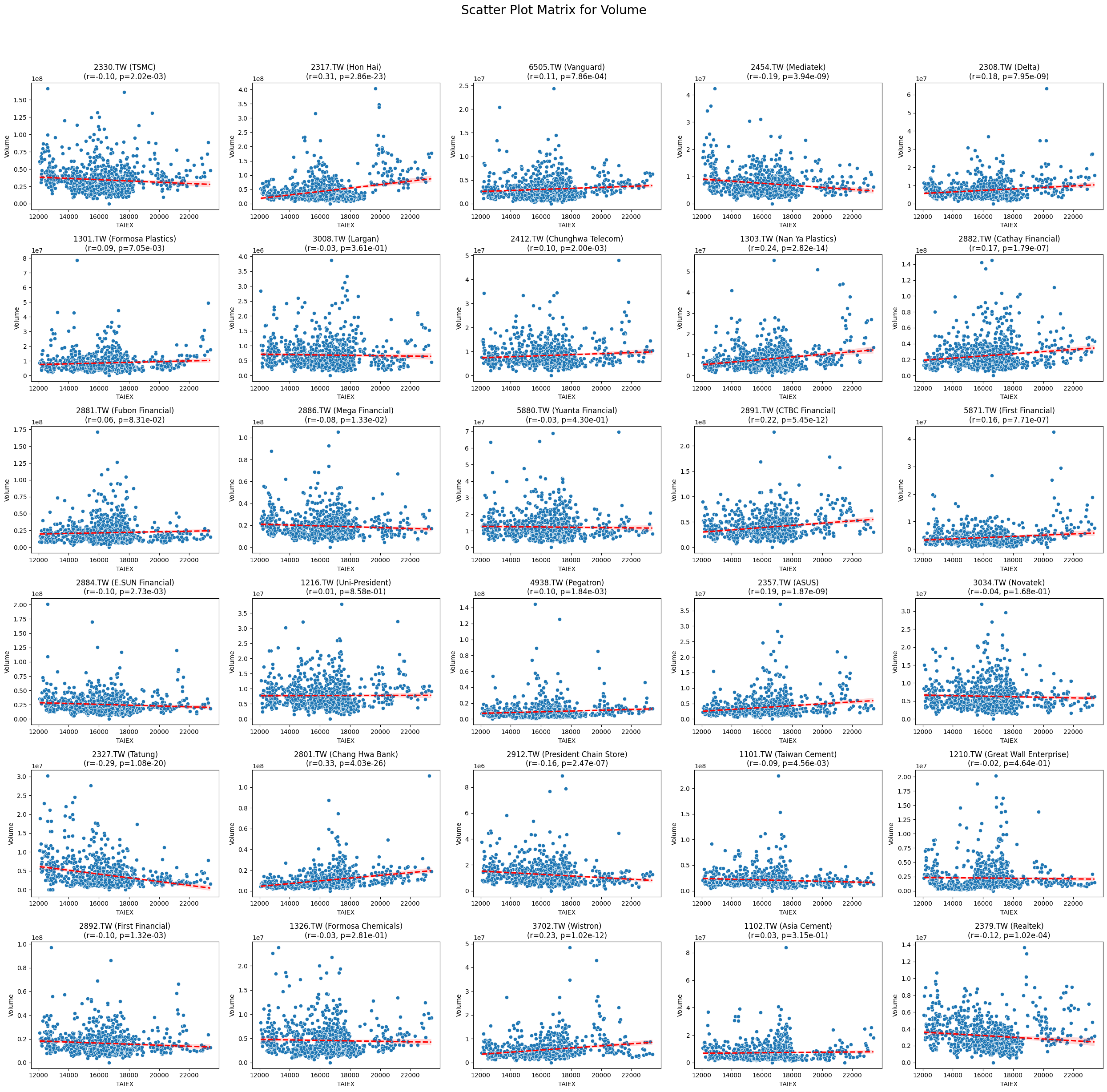
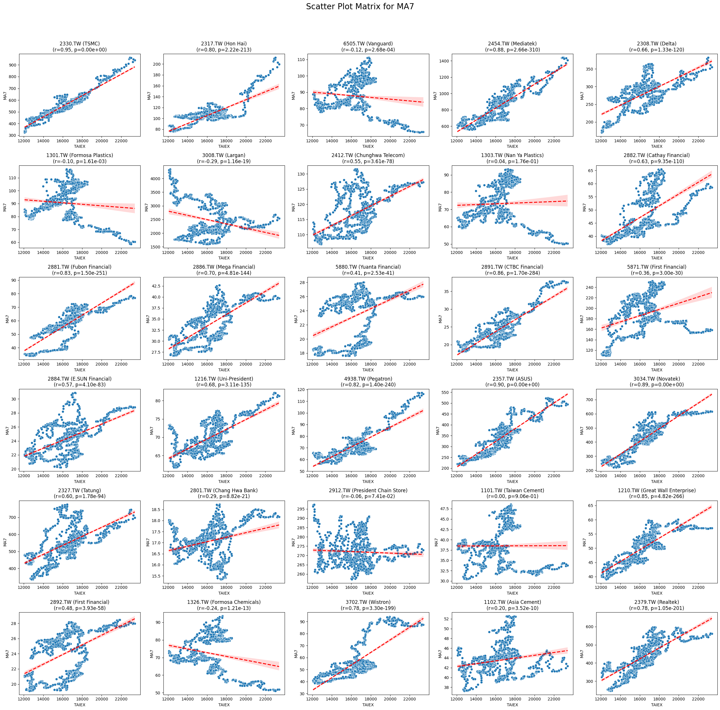
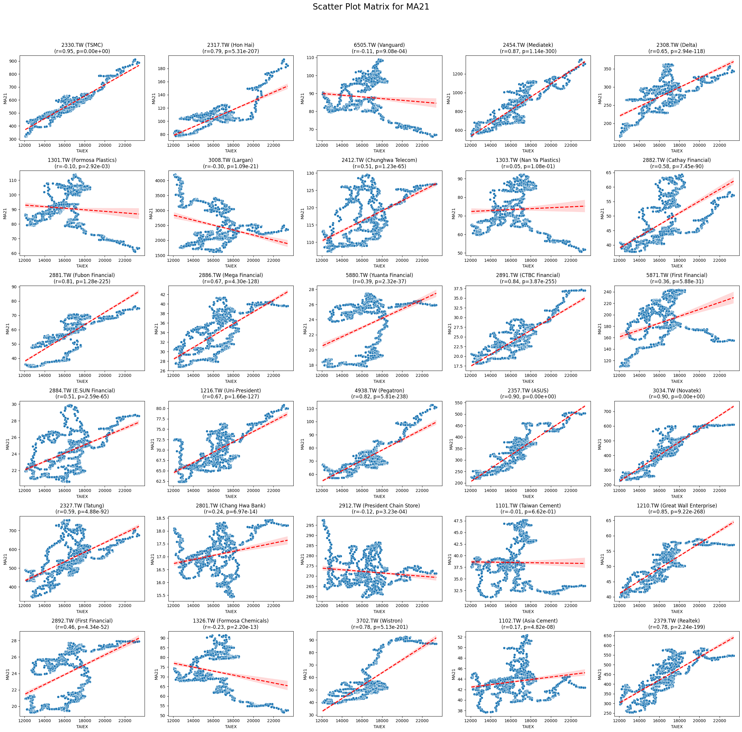
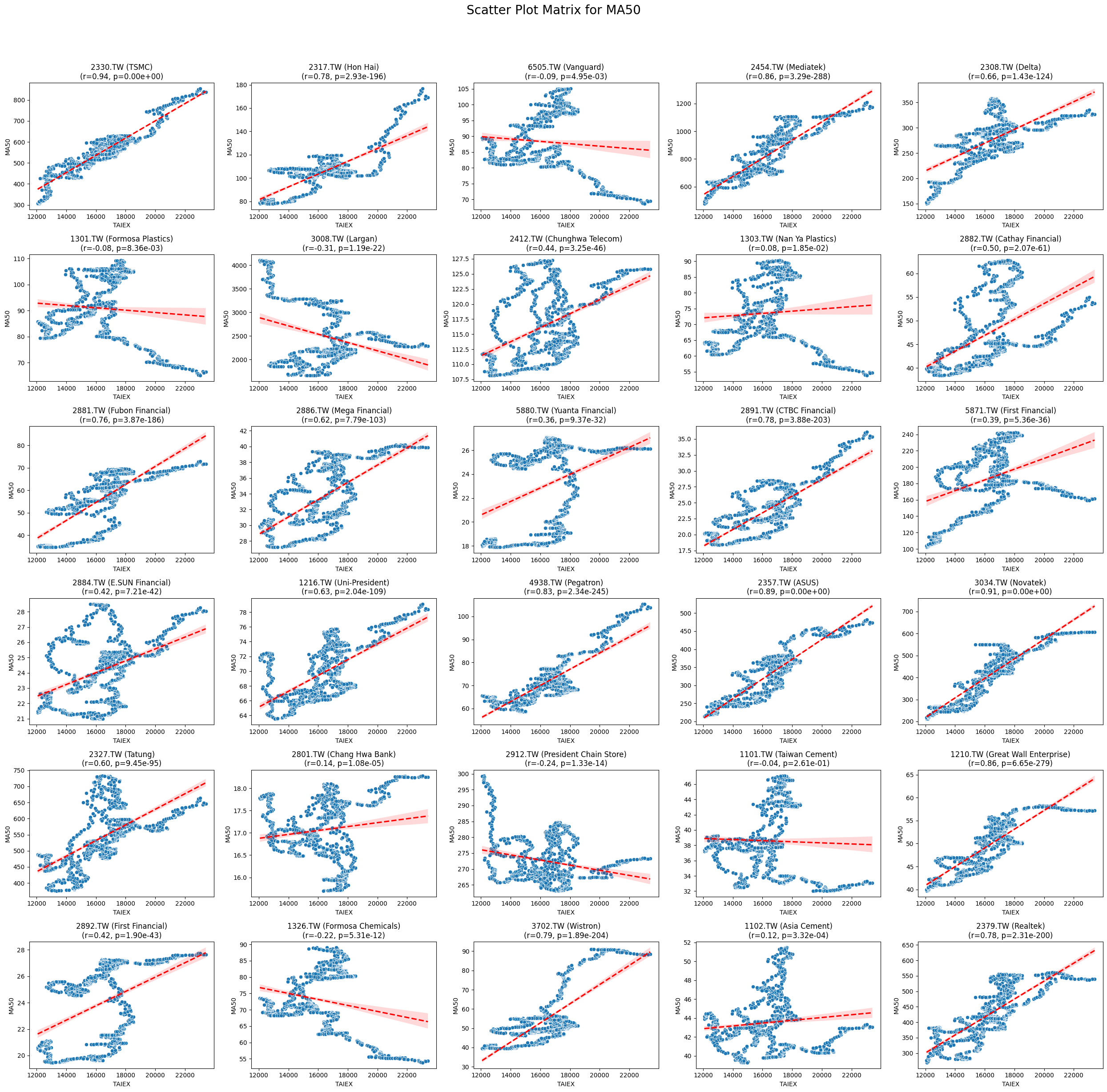
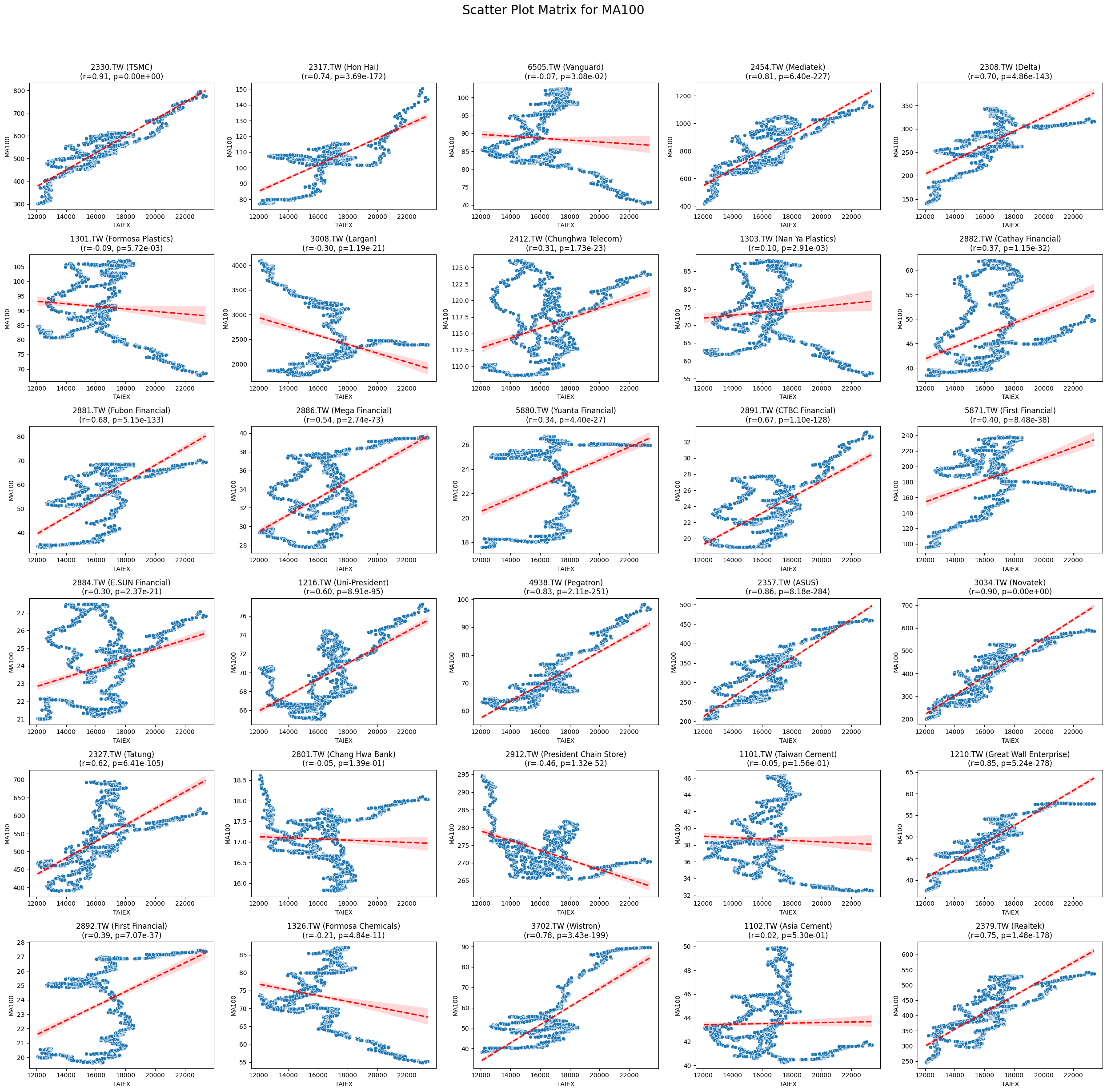
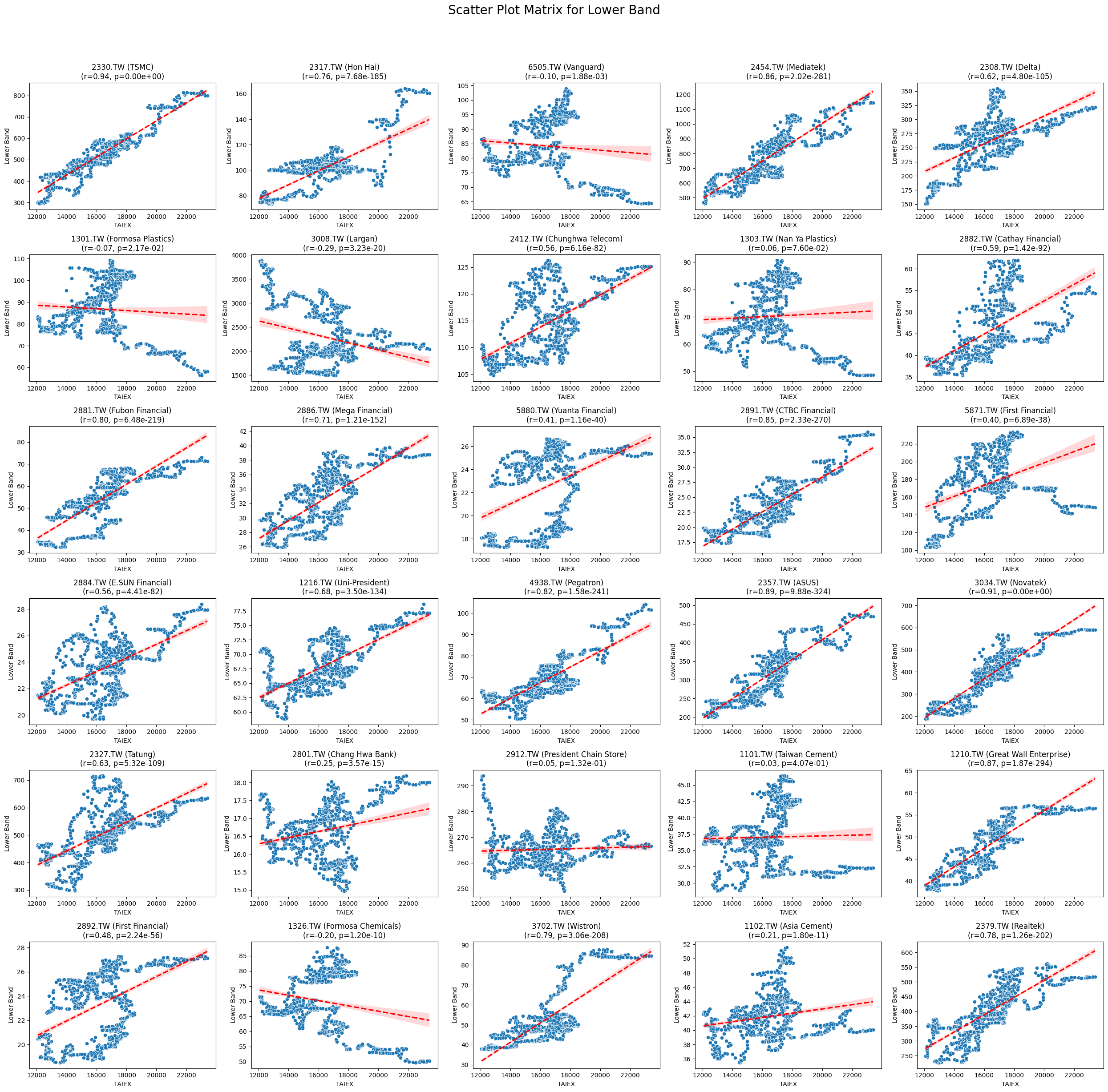
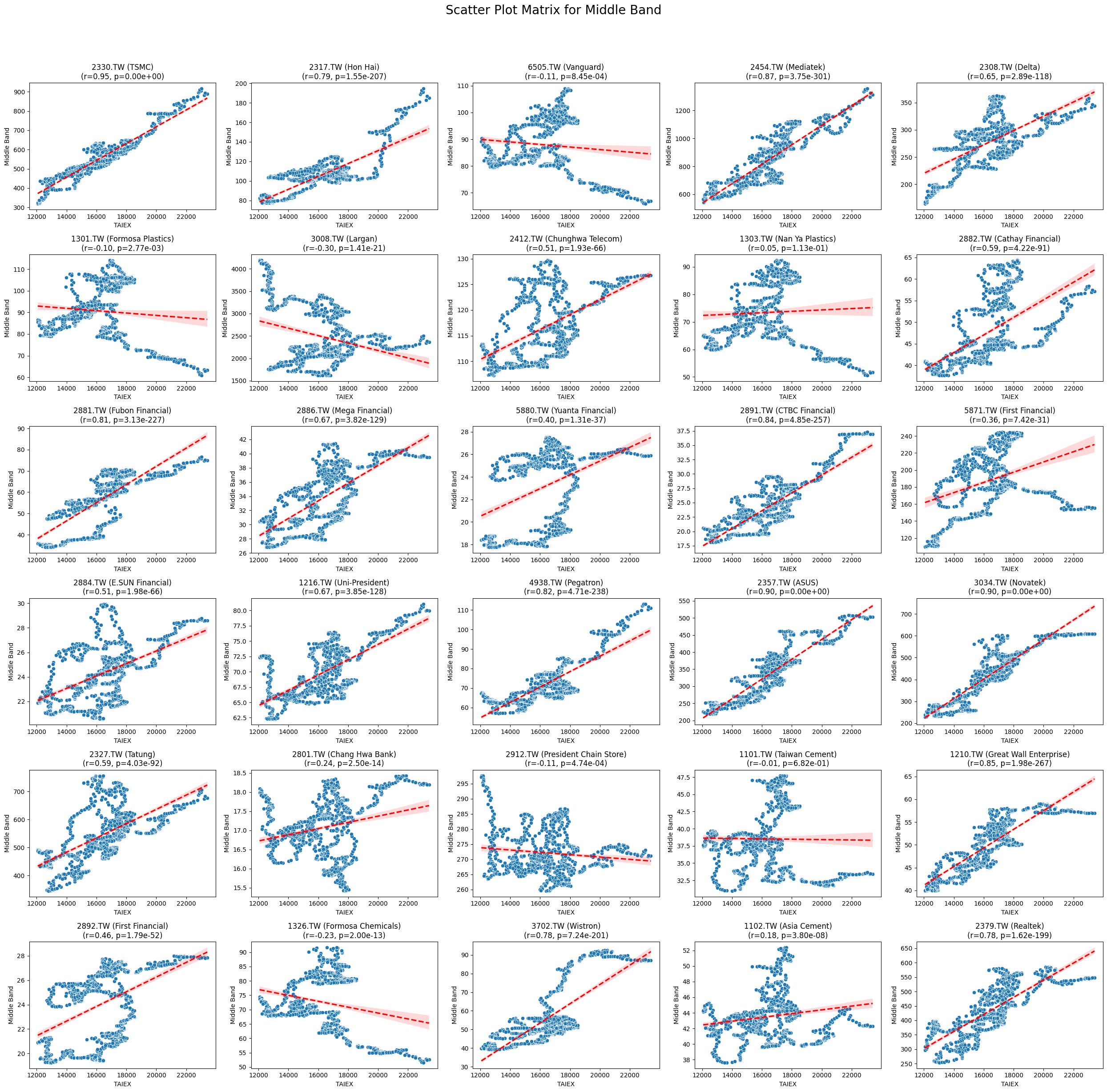
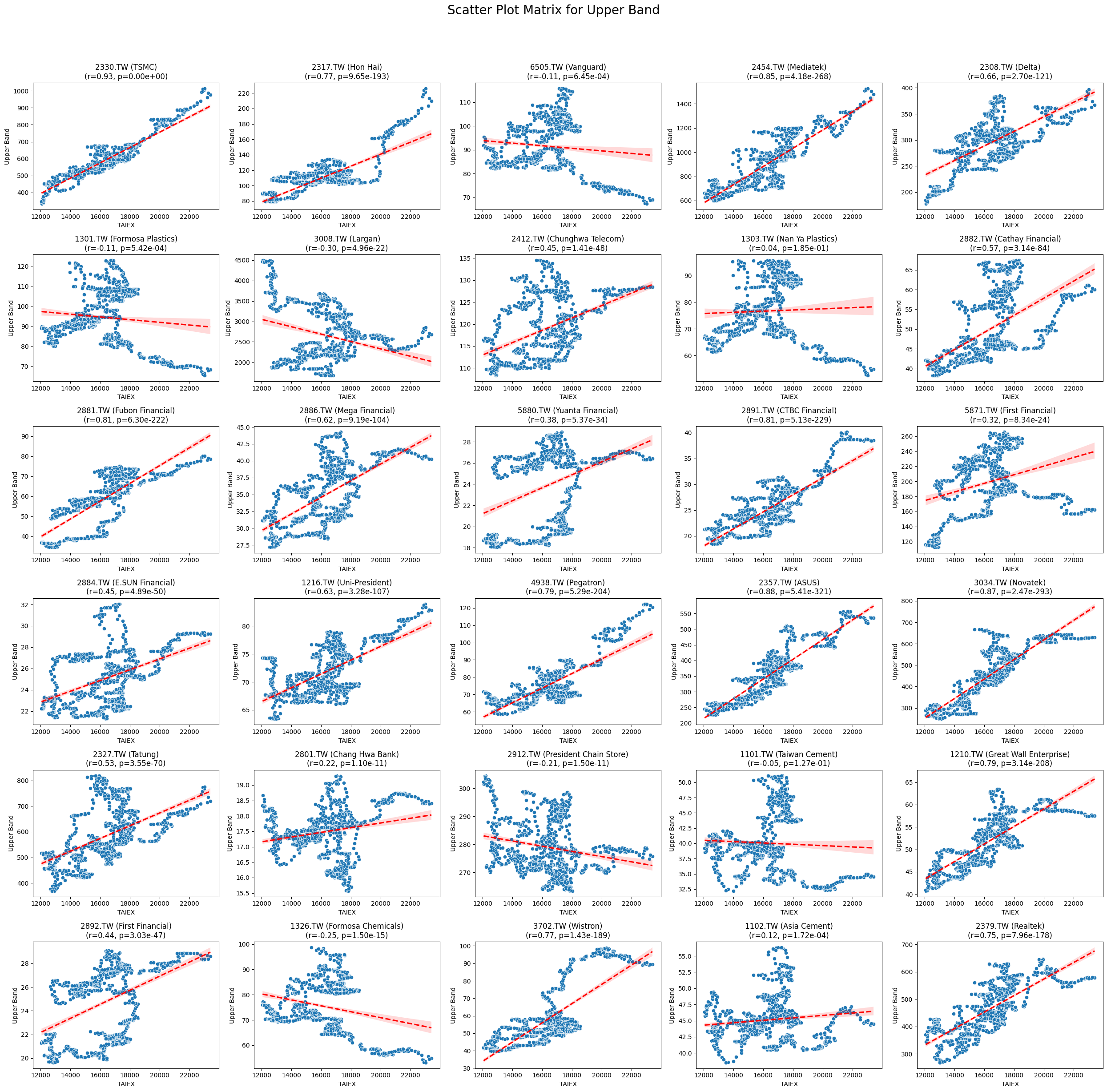
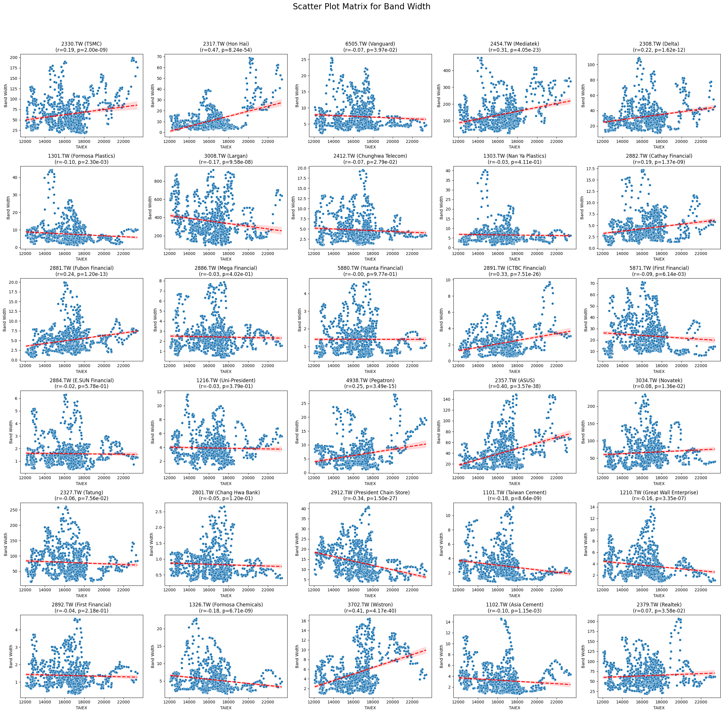
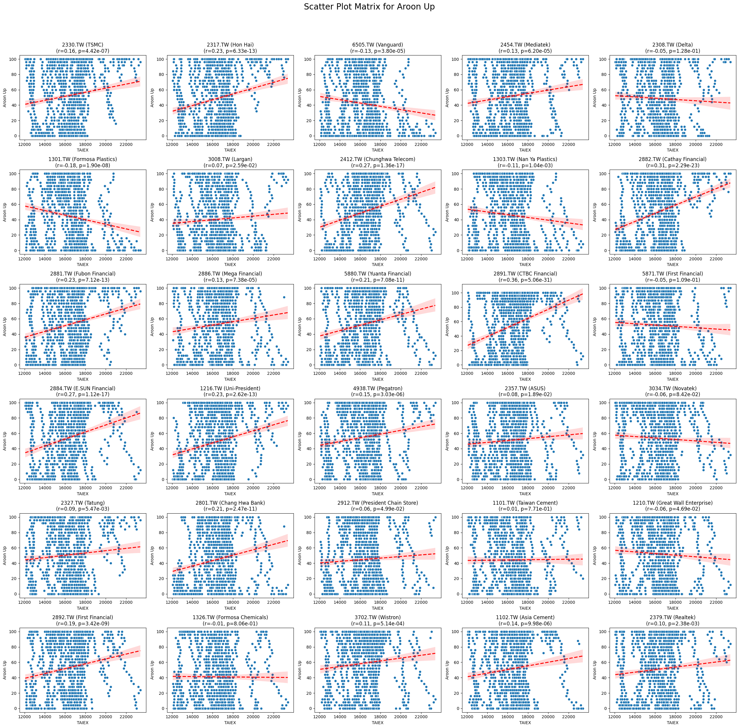
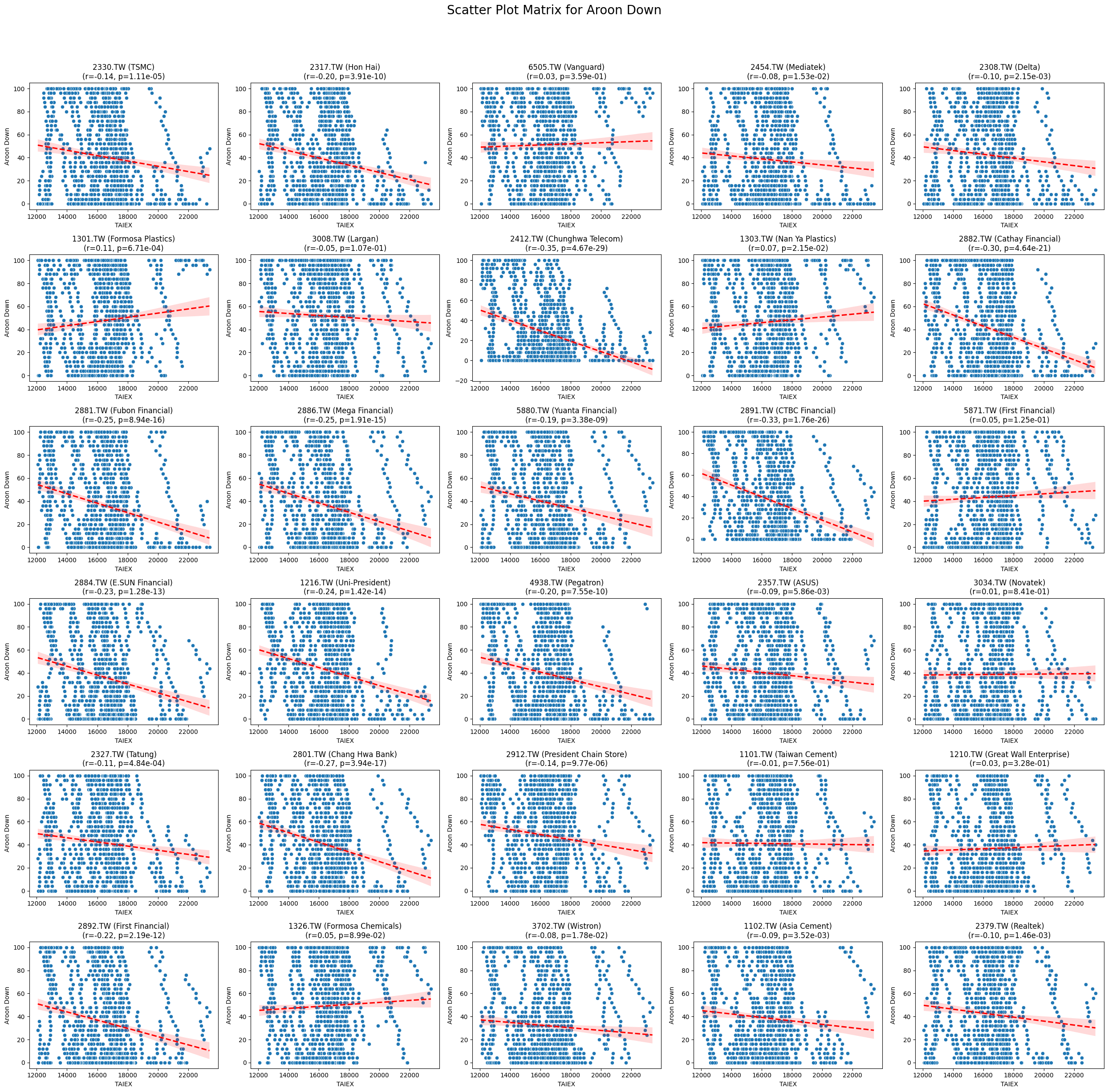
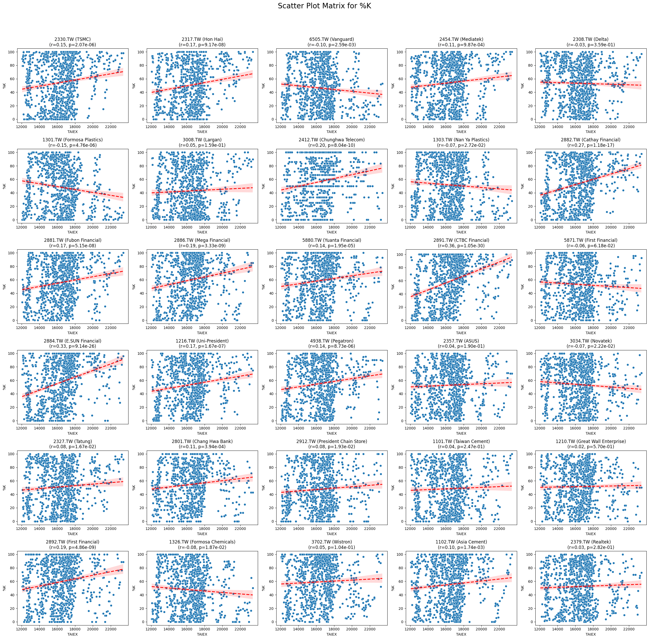
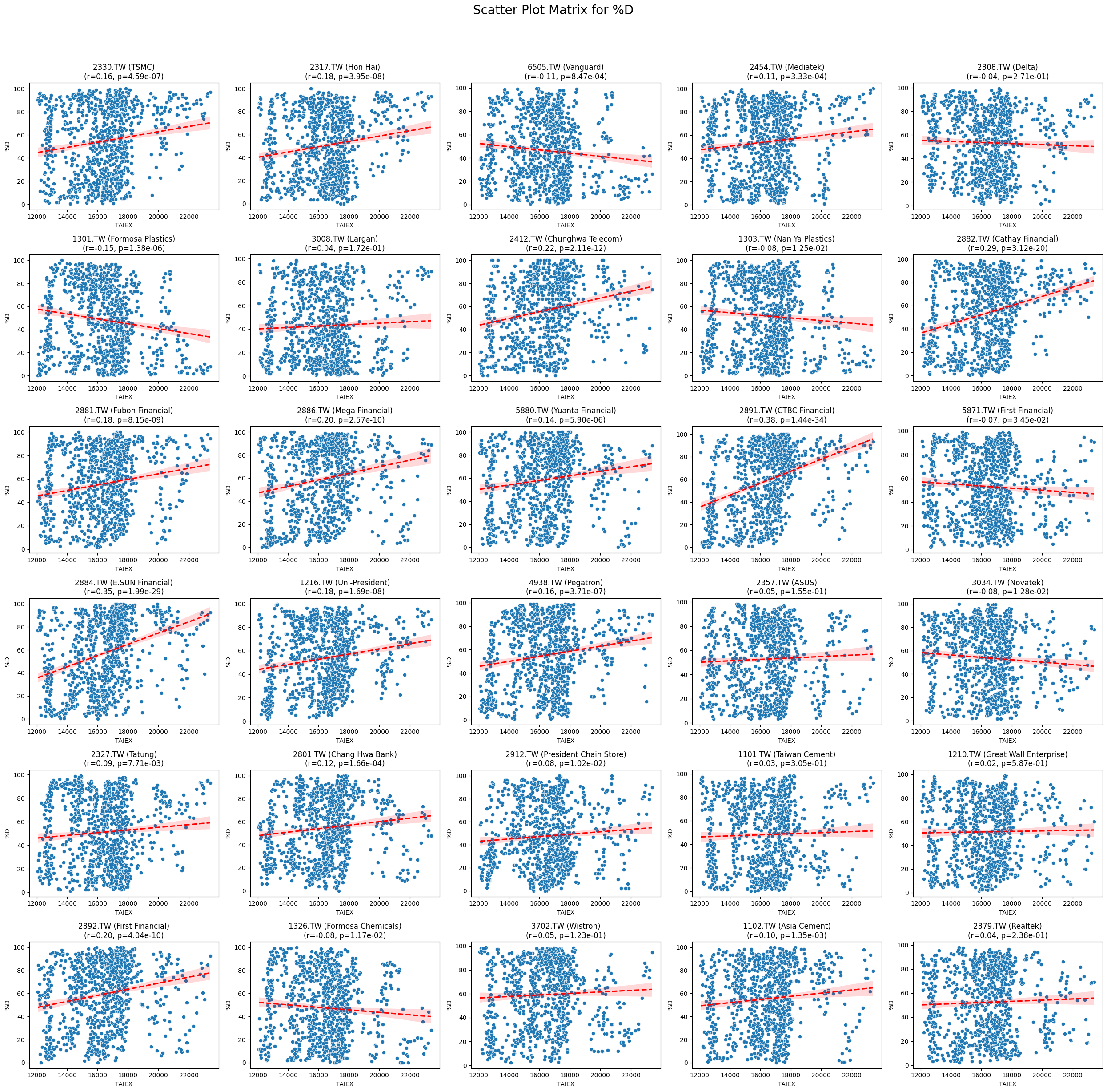
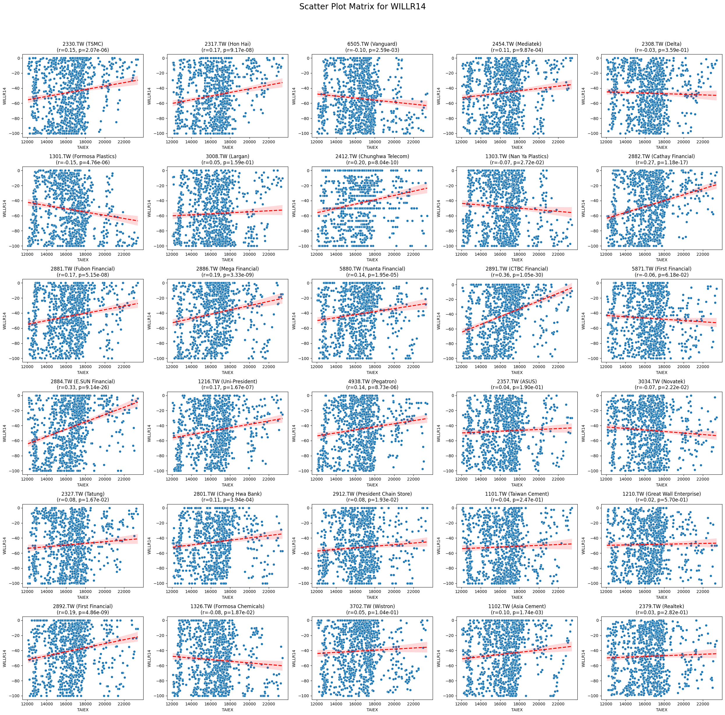
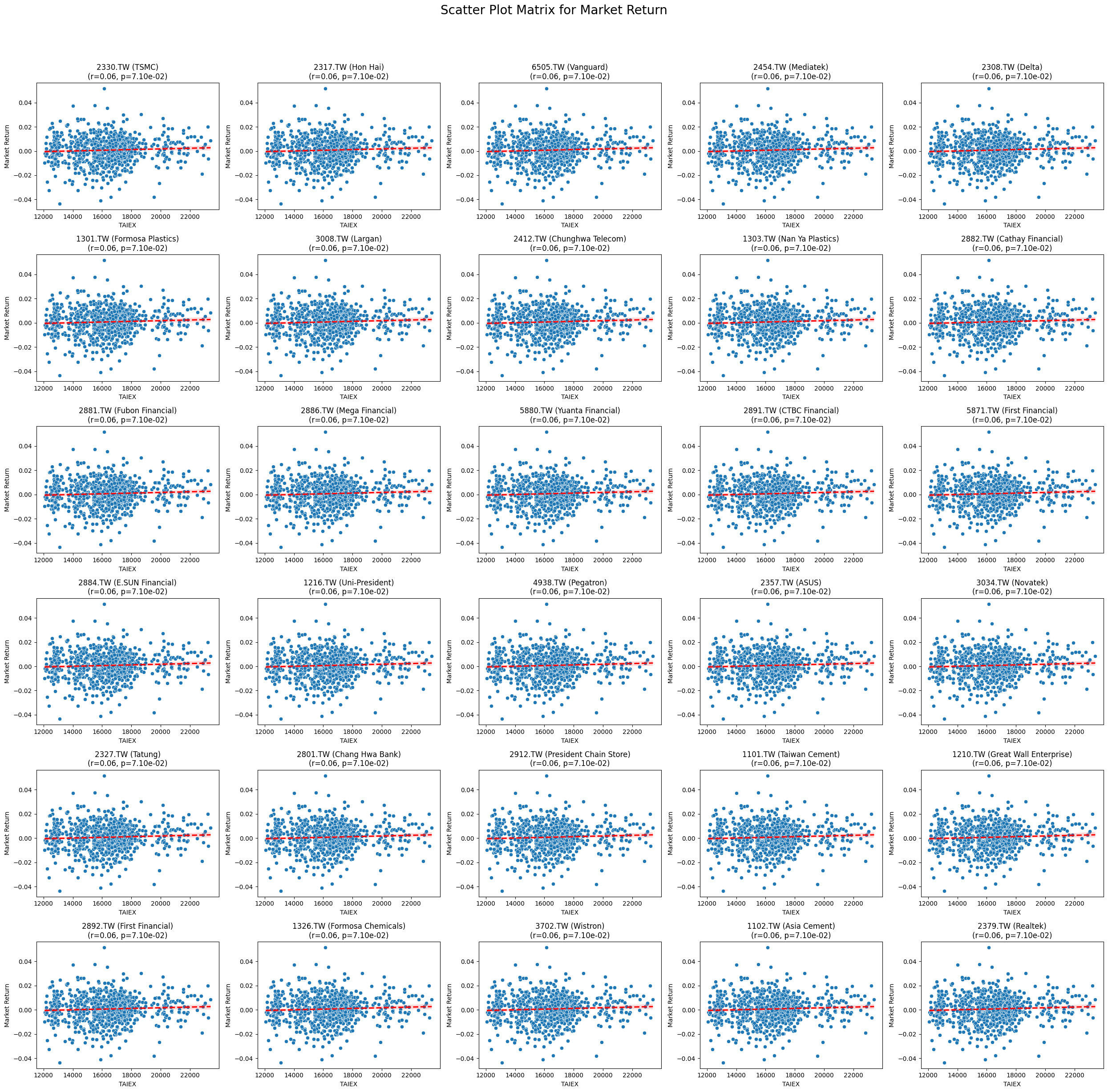
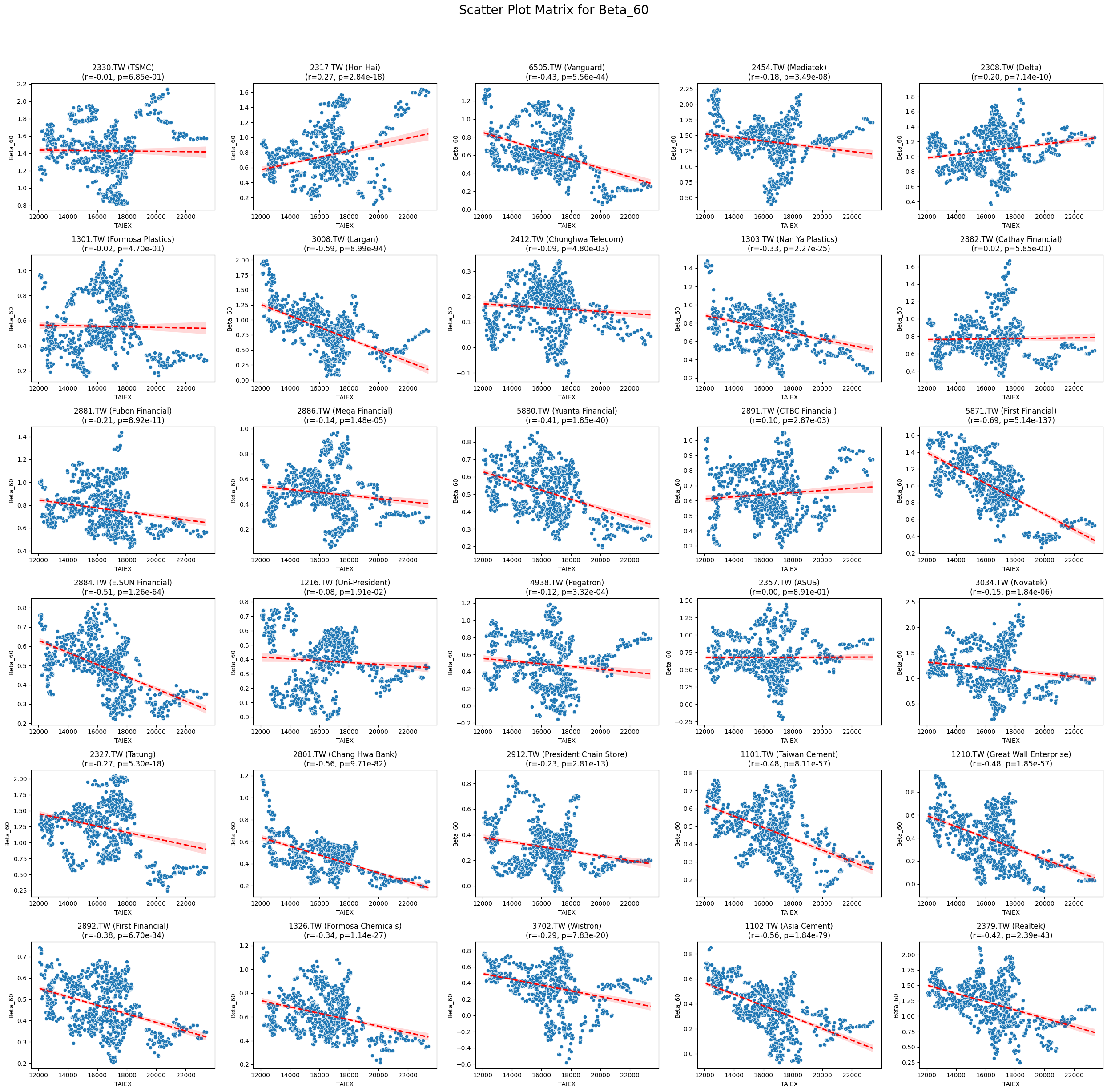
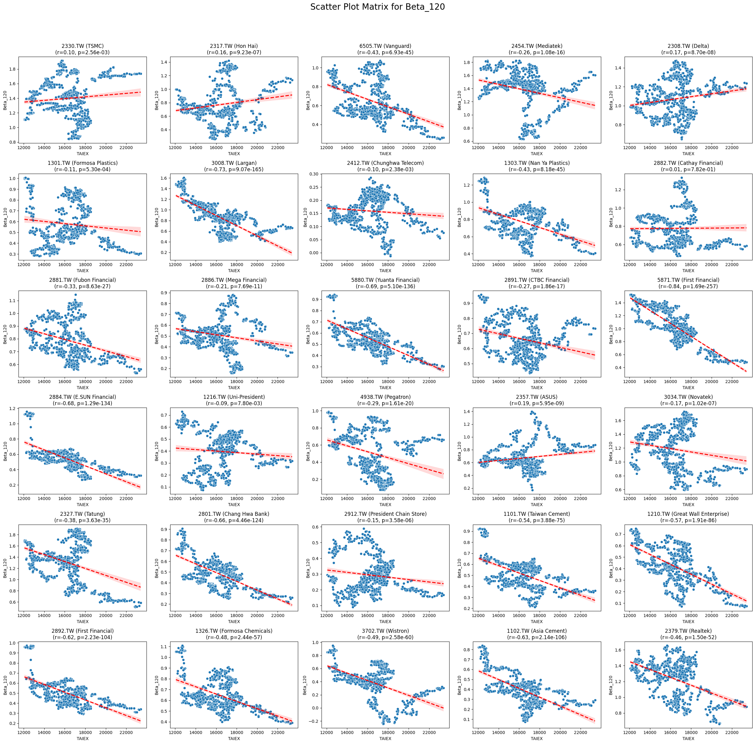
# Function to create scatter plot matrix by variable
def scatter_plot_matrix_by_variable():
variables = [col for col in data.columns if col not in ['Date', 'ST_Code', 'ST_Name', target_variable]]
for variable in variables:
plt.figure(figsize=(25, 25))
unique_stock_codes = data['ST_Code'].unique()
for i, stock_code in enumerate(unique_stock_codes):
stock_data = data[data['ST_Code'] == stock_code]
taiex_data = data[['Date', target_variable]].drop_duplicates()
aligned_data = pd.merge(stock_data, taiex_data, on='Date', suffixes=('', '_TAIEX'))
aligned_data = aligned_data.replace([np.inf, -np.inf], np.nan).dropna()
if aligned_data.shape[0] > 0 and variable in aligned_data.columns:
correlation, p_value = pearsonr(aligned_data[target_variable], aligned_data[variable])
plt.subplot((len(unique_stock_codes) + 4) // 5, 5, i + 1)
sns.scatterplot(x=aligned_data[target_variable], y=aligned_data[variable])
sns.regplot(x=aligned_data[target_variable], y=aligned_data[variable], scatter=False, color='red', ci=95, line_kws={'linestyle': 'dashed'})
stock_name = aligned_data['ST_Name'].iloc[0] # Get the stock name from the first row
plt.title(f'{stock_code} ({stock_name})\n(r={correlation:.2f}, p={p_value:.2e})')
plt.xlabel('TAIEX')
plt.ylabel(variable)
plt.suptitle(f'Scatter Plot Matrix for {variable}', fontsize=20)
plt.tight_layout(rect=[0, 0, 1, 0.95])
plt.savefig(f'/content/drive/My Drive/scatter_plot_matrix_{variable}.png')
plt.show()
# Generate scatter plot matrix by variable
scatter_plot_matrix_by_variable()import pandas as pd import yfinance as yf import ta from datetime import datetime